Spatial SQL with PostgreSQL and PostGIS

PostgreSQL and PostGIS let you store, query, edit, and analyze spatial data directly inside a database. Instead of exporting layers into a desktop GIS for every operation, many workflows — buffering, spatial joins, dissolves, reprojection, and validation — run as SQL. This post introduces the core concepts you need to start writing spatial SQL, working a Natural Earth dataset from installation through to query optimization.

Why bother? Most GIS work treats the database as a passive place to park data: you pull features into a desktop tool, run geoprocessing, and push results back. Moving that work into the database changes the economics. Joins, buffers, dissolves, and reprojections become single statements that run on a schedule, integrate with other systems, and stay close to the data.

This post walks through the core ideas of spatial SQL using PostgreSQL and PostGIS. It follows the structure of John Reiser’s Spatial SQL workshop; the workshop data, installers, and updates are at learnspatialsql.com.

This is a summary and reference, not a substitute for a live environment. Install the software, load the workshop data, and run the queries yourself. The concepts only stick when you type them.

What You Need

A typical PostGIS environment consists of five components:

• PostgreSQL — an open-source, ACID-compliant relational database for Windows, macOS, and Linux. Version 16 or later is preferred; 13+ works. Avoid any end-of-life version, since it no longer receives security patches.
• PostGIS — the spatial extension that adds geometry storage, spatial functions, and spatial indexing.
• A SQL client — this post uses pgAdmin 4, which is Postgres-specific. DBeaver and psql are common alternatives.
• A desktop GIS — QGIS (open source) or ArcGIS Pro, to see the geometry as a map alongside the tabular view.
• The workshop data — a Natural Earth subset delivered as a PostgreSQL dump.

Platform notes:

• On Windows, the EnterpriseDB installer bundles Stack Builder, which is where you add PostGIS. Select it during install.
• On macOS, Postgres.app is the simplest route and ships with PostGIS already installed.

Postgres.app is fine for learning but is explicitly not recommended for production use.

When installing, you set a password for the postgres superuser. That account is convenient for a workshop because it can do anything, which is exactly why it is dangerous in production.

Operating as postgres (or any superuser) in a production database without understanding the consequences can destroy data with a single statement. In a real deployment, work with a DBA to define proper users, roles, and permissions.

Enabling PostGIS in a database is a one-liner:

CREATE EXTENSION postgis;

How a Database Is Organized

A relational database nests objects. Reading from the smallest unit outward:

• A record is one item — say, a US state — made of properties like name, population, and shape.
• A column holds one property across records.
• A table is a set of records sharing the same columns. The column definition is the table’s schema (in the structural sense).
• A schema (in the PostgreSQL sense) is a named grouping of tables, views, functions, and types inside a database. SQLite has no equivalent, because it is single-user.
• A database is a collection of schemas and tables.
• A server instance is the running PostgreSQL process. It listens for connections, enforces access control, and manages the data on disk.
• A database cluster, in PostgreSQL’s own terminology, is the collection of databases managed by a single server instance — the storage that initdb creates. One instance manages exactly one cluster.

So the containment runs from the process down to a single row:

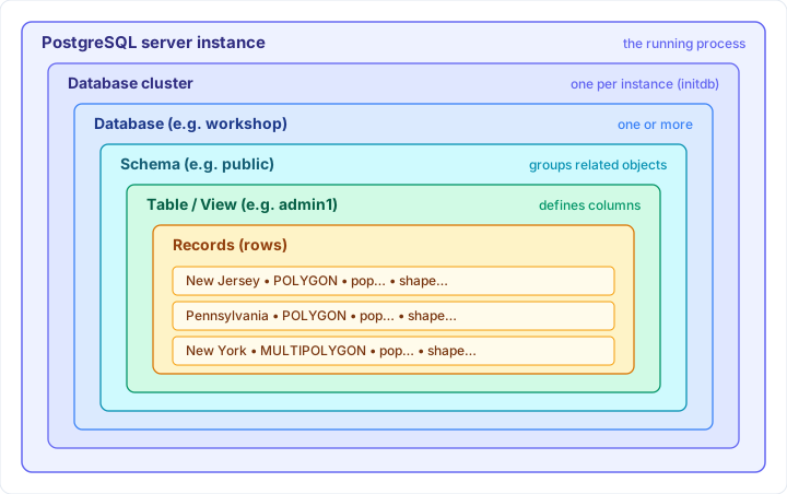Each level contains all of the elements of the next: an instance manages one cluster, a cluster holds databases, a database holds schemas, a schema holds tables and views, and a table holds records.

The word cluster is overloaded. In high-availability discussions it often means several cooperating servers behind a load balancer. In the PostgreSQL documentation it means the databases managed by one instance, which is the sense used here.

Data moves freely between schemas in one database. Moving data between databases requires an explicit connection — pg_dump/pg_restore for snapshots, or Foreign Data Wrappers for live links (covered below).

ACID, briefly

The guarantees that make a database trustworthy:

• Atomicity — changes in a transaction persist only when committed; otherwise they roll back.
• Consistency — invalid data causes the transaction to roll back.
• Isolation — concurrent transactions don’t corrupt one another.
• Durability — a committed change stays until another committed change replaces it.

Most clients auto-commit, wrapping each statement in its own transaction. Use BEGIN, COMMIT, and ROLLBACK to group statements into a single unit.

Speaking SQL

SQL is a declarative language: you state the result you want, and the query planner decides how to produce it. That is a different mindset from Python or Java.

If you have used ArcGIS Select By Attributes, you have already written SQL — the box at the bottom of that dialog is a WHERE clause on SELECT * FROM table_name.

The clauses available in a SELECT statement:

SELECT
FROM
JOIN
WHERE
GROUP BY
HAVING
ORDER BY
LIMIT

They are written in that order but executed in a different one:

1. FROM / JOIN
2. WHERE
3. GROUP BY
4. HAVING
5. SELECT
6. ORDER BY
7. LIMIT

Although a query is written starting with SELECT, the database first decides where the data comes from (FROM and any JOINs), filters rows (WHERE), groups them (GROUP BY), and only then builds the output columns (SELECT) before sorting and limiting. Keeping that flow in mind explains several errors that otherwise look arbitrary.

This execution order matters as queries grow. Column aliases created in SELECT, for example, don’t exist yet when WHERE runs — a common source of “column does not exist” errors. Violating the order also produces slow or invalid queries.

Building up a query

Start with everything, then narrow. Using the workshop’s public.admin1 table (states and provinces):

SELECT * FROM public.admin1;

Limit columns and rows, sort, and deduplicate:

SELECT DISTINCT sov_a3, geonunit, name
  FROM public.admin1
 WHERE iso_a2 = 'US'
 ORDER BY 1, 2, 3;

A few things worth noting:

• ORDER BY 1, 2, 3 sorts by column position (counting from 1 on the left). Handy, but explicit column names are clearer.
• DISTINCT returns a unique set of rows.
• Columns used in WHERE do not have to appear in the SELECT list.

Geometry Is Just Another Column

Select a geometry directly and you get an unreadable string — that’s Well-Known Binary (WKB):

SELECT name, shape
  FROM public.admin1
 WHERE name = 'New Jersey';

A geometry column stores a shape together with the type that shape takes. The common types map cleanly onto GIS features:

Geometry type	Typical feature
POINT	a city or sample site
LINESTRING	a road or river
POLYGON	a state or parcel
MULTIPOLYGON	a country with islands

PostGIS also offers a separate geography type. geometry treats coordinates as points on a flat plane — fast, and supported by the full function library. geography treats them as points on the WGS84 spheroid, so distances and areas come back in meters measured on the curved Earth. Use geometry in a projected coordinate system for most analysis, and reach for geography when you need accurate global measurements without picking a projection.

PostGIS functions translate geometry into readable formats. ST_AsEWKT() and ST_AsGeoJSON() both take geometry and return text:

SELECT name, ST_AsEWKT(shape)
  FROM public.admin1
 WHERE name = 'New Jersey';

SELECT name, ST_AsGeoJSON(shape)
  FROM public.admin1
 WHERE name = 'New Jersey';

Every geometry carries a Spatial Reference ID (SRID) that identifies its coordinate system. Most SRIDs are EPSG codes: 4326 is WGS84 (longitude/latitude in degrees), and 3424 is New Jersey State Plane (feet). The full definitions live in public.spatial_ref_sys, and ST_SRID(shape) reports the SRID of any value.

Functions nest, and because each expects a specific input type and returns a specific type, the call order matters. ST_Transform() reprojects a geometry to a target SRID — here, New Jersey State Plane (3424):

SELECT name,
       ST_AsEWKT( ST_Transform(shape, 3424) ) AS stateplane,
       ST_AsEWKT( shape )                      AS latlng
  FROM public.admin1
 WHERE name = 'New Jersey';

You can list a column more than once and alias each result — here, the same shape in State Plane and in native WGS84.

ST_Centroid() returns the center point of a line or polygon, and since it returns geometry, it feeds straight into other geometry functions.

To see what spatial data a database holds, query the geometry_columns view: SELECT * FROM geometry_columns; lists every geometry column with its type and SRID. Find_SRID('public', 'admin1', 'shape') returns the SRID registered for a single column.

Making New Tables from Queries

Create a schema to keep your own objects separate from the reference data:

CREATE SCHEMA workspace;

Add it to the search path so you can reference mytable instead of workspace.mytable:

ALTER DATABASE workshop SET search_path = "$user", workspace, public;

"$user" tells the planner to check a schema matching the current user’s name first. It’s good practice once a database has multiple users.

Search-path order matters. If workspace precedes public and both contain an admin1 table, an unqualified admin1 resolves to workspace.admin1.

Any valid SELECT becomes a table with CREATE TABLE ... AS:

CREATE TABLE workspace.usplaces AS
  SELECT id, shape, name,
         adm1name AS state,
         pop_max, pop_min, pop_other,
         max_areami AS areasqmi,
         elevation, timezone
    FROM public.places
   WHERE iso_a2 = 'US';

This copies the rows once — a static snapshot. If public.places changes later, usplaces does not follow. When you want a result that always reflects its source, use a view instead (next section).

SELECT happily returns unnamed columns, but CREATE TABLE AS requires every column to have a name. Alias any computed or renamed column.

Aggregates and views

GROUP BY with aggregate functions computes statistics per group:

SELECT state, count(*), sum(pop_max)
  FROM workspace.usplaces
 GROUP BY state
 ORDER BY state;

A view stores a query, not data — it references the underlying tables each time it’s called. The syntax mirrors CREATE TABLE AS:

CREATE VIEW workspace.placestats AS
  SELECT state, count(*), avg(pop_max)
    FROM workspace.usplaces
   GROUP BY state;

PostGIS adds spatial aggregates. ST_Union() with GROUP BY performs the equivalent of an ArcGIS dissolve, merging geometries within each group:

CREATE OR REPLACE VIEW workspace.usregions AS
  SELECT min(id) AS objectid,
         ST_Union(shape) AS shape,
         region
    FROM admin1
   WHERE iso_a2 = 'US'
   GROUP BY region;

min(id) supplies a stable, unique key per group so a GIS client has something to use as an ObjectID. Grouping by a unique column would defeat the merge, so aggregate the key with min() or max() instead.

Types Are Not Optional

Functions dispatch on input type and return a type based on the input. Getting types wrong produces silently wrong results.

The classic trap:

SELECT 1/4;   -- returns 0, integer division

Force numeric math with any of:

SELECT 1.0/4.0;
SELECT 1::numeric / 4::numeric;
SELECT 1/4.0;   -- a single decimal operand is enough

Order of operations bites when combined with type modifiers:

SELECT (1.0/4.0)::numeric(3,2);   -- 0.25
SELECT (1/4)::numeric(3,2);       -- 0.00  (integer division happens first)

Dates and CAST

Sorting a text column that holds dates sorts lexically, not chronologically. Convert explicitly with CAST() or the :: shorthand:

SELECT * FROM public.us_state_info
 ORDER BY CAST(statehood AS date);

Comparisons need both operands to be the same comparable type. This fails:

SELECT * FROM public.us_state_info WHERE statehood > 1875;
-- ERROR: operator does not exist: text > integer

This works:

SELECT * FROM public.us_state_info
 WHERE statehood::date > '1875-12-31'::date;

Always write dates in unambiguous ISO 8601 form: YYYY-MM-DD, eight digits, zero-padded. 04/06/12 could mean three different dates depending on locale.

Joining Tables

An inner join returns the subset of the Cartesian product where a comparison holds. Aliases keep it readable:

SELECT a.id, a.shape, a.name, a.region, a.postal,
       i.statehood::date AS statehood,
       i.capital, i.largestcity, i.population, i.houseseats
  FROM public.admin1 a
  JOIN public.us_state_info i
    ON a.postal = i.abbr
 WHERE a.iso_a2 = 'US';

The WHERE a.iso_a2 = 'US' filter matters: without it, a state postal code like MN can match provinces in other countries.

These two forms are equivalent, but prefer the explicit JOIN:

-- explicit (recommended)
SELECT x.col1, y.col2 FROM table1 x JOIN table2 y ON x.key = y.key;

-- implicit
SELECT x.col1, y.col2 FROM table1 x, table2 y WHERE x.key = y.key;

The explicit form gives clearer errors when something is wrong.

A primary key does not follow a column into a new table. Add it after the fact:

ALTER TABLE workspace.usstates ADD PRIMARY KEY (id);

Spatial joins

Instead of matching on a shared value, a spatial join matches on a spatial relationship. ST_Contains(a, b) returns TRUE when a contains b, so it can serve as a join predicate — counting the place points in each state:

SELECT s.name, s.shape, COUNT(p.shape)
  FROM usstates s
  JOIN usplaces p ON ST_Contains(s.shape, p.shape)
 GROUP BY s.name, s.shape;

Before running a join, know the row counts of both inputs. If usstates has 51 rows and usplaces has 769, an unrestricted cross join produces 39,219 rows. A result of zero means your join columns share no matching values. Use the returned count as a sanity check.

ST_Contains() is one of a family of spatial predicates, each returning a boolean you can use as a join or WHERE condition:

Function	Returns true when…
ST_Intersects(a, b)	a and b share any point at all
ST_Contains(a, b)	a completely contains b
ST_Within(a, b)	a lies completely inside b
ST_Touches(a, b)	they share a boundary but no interior
ST_Overlaps(a, b)	they overlap, but neither fully contains the other
ST_Disjoint(a, b)	they share no point (the opposite of ST_Intersects)

ST_Contains and ST_Within are mirror images: ST_Contains(a, b) is the same test as ST_Within(b, a).

Indexes and EXPLAIN

Spatial predicates are far more expensive than integer comparisons, and every join risks evaluating a large slice of the Cartesian product. Indexes let the planner skip irrelevant rows.

Prefix any query with EXPLAIN to see the plan:

EXPLAIN
SELECT s.name, s.shape, COUNT(p.shape)
  FROM usstates s
  JOIN usplaces p ON ST_Contains(s.shape, p.shape)
 GROUP BY s.name, s.shape;

The word to hunt for is Seq Scan — a full sequential scan, which gets painful on large tables and expensive functions.

PostGIS accelerates spatial columns with a GiST (Generalized Search Tree) index. It stores each geometry’s bounding box in a tree, so the planner can discard the vast majority of rows with a cheap box comparison before it runs the exact, expensive predicate such as ST_Contains(). Build one on both geometry columns:

CREATE INDEX ON workspace.usstates USING gist(shape);
CREATE INDEX ON workspace.usplaces USING gist(shape);

Re-run EXPLAIN and the sequential scan on usplaces becomes an Index Scan, with the plan’s cost figures dropping sharply. The planner may still scan a tiny table (51 rows) sequentially because that’s genuinely cheaper.

Indexes trade storage for speed. That trade is almost always worth it — storage is cheap relative to the query time a spatial index saves.

EXPLAIN output is dense. Tools like explain.depesz.com visualize the plan and highlight the expensive steps.

Updating Data with a Spatial Join

usplaces.timezone has 77 NULLs:

SELECT COUNT(*) FROM usplaces WHERE timezone IS NULL;

The public.timezones table has timezone polygons and a matching tz_name. An UPDATE can fill the gaps using a spatial relationship as the join condition:

UPDATE usplaces p
   SET timezone = t.tz_name
  FROM public.timezones t
 WHERE ST_Contains(t.shape, p.shape)
   AND p.timezone IS NULL;

Two conditions: the spatial one defines which timezone polygon each point falls in, and p.timezone IS NULL restricts the update to rows that actually need it. Re-run the count and it returns 0.

You created usplaces in your own schema, so you can modify it. You don’t have permission to alter tables in public, so the worst case is dropping and recreating your own tables.

Creating New Geometry from Intersections

Two similarly named functions do different jobs:

• ST_Intersects(a, b) — returns a boolean: do the geometries touch at all?
• ST_Intersection(a, b) — returns the geometry of the overlapping area (NULL if they don’t intersect).

Test with the boolean, build with the geometry. Intersecting states with timezones produces split pieces where a state spans two zones, so no existing primary key stays unique. A temporary sequence generates fresh IDs:

CREATE TEMPORARY SEQUENCE newid START WITH 1;

CREATE TABLE ustimezones AS
  SELECT nextval('newid') AS id,
         ST_Intersection(s.shape, tz.shape) AS shape,
         s.name, s.region, s.postal,
         tz.zone, tz.tz_name, tz.utc_format
    FROM usstates s, public.timezones tz
   WHERE ST_Intersects(s.shape, tz.shape);

ALTER TABLE ustimezones ADD PRIMARY KEY (id);

A temporary sequence disappears when you disconnect, so there’s nothing to clean up. The result is 80 rows — more than 51 states, because zone-split states get one row per piece.

Materialized Views

A regular view runs its query every time. A materialized view stores the results on disk, so reads are as fast as a single-table lookup and you can index it. The cost is storage plus manual refresh:

CREATE MATERIALIZED VIEW mv_data_2024 AS SELECT ...;
REFRESH MATERIALIZED VIEW mv_data_2024;

REFRESH MATERIALIZED VIEW CONCURRENTLY keeps the view readable during a refresh, but requires a unique index on the view.

A common pattern wraps a materialized view in a plain view, letting you swap the underlying materialized view without clients noticing:

CREATE MATERIALIZED VIEW mv_data_2024 AS SELECT ...;
CREATE OR REPLACE VIEW v_last_year_data AS SELECT * FROM mv_data_2024;

Materialized views also help with permissions — a view can expose a controlled slice of sensitive tables — and with snapshotting data as of a point in time.

Foreign Data Wrappers

Foreign Data Wrappers (FDW) present external sources as if they were local tables. There are wrappers for other databases (Oracle, SQL Server, MySQL), for files (CSV, Excel), and — via the ogr_fdw extension that ships with PostGIS — for spatial services like GeoJSON APIs, WFS, and ArcGIS REST endpoints.

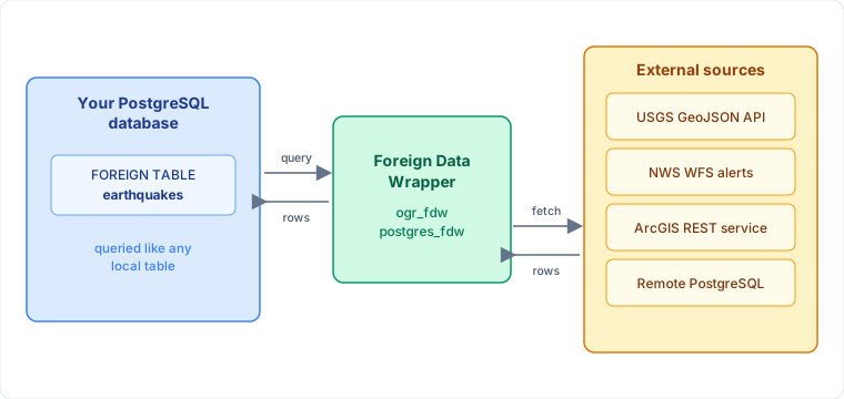A foreign table looks local, but every query is routed through the wrapper to a live external source.

ogr_fdw relies on GDAL/OGR, and getting those libraries working reliably on Windows can be difficult. The linked AWS Windows instance in the workshop is pre-configured if you hit trouble.

Wrapping the USGS earthquake feed takes a foreign server plus a foreign table:

CREATE EXTENSION ogr_fdw;

CREATE SERVER usgs
  FOREIGN DATA WRAPPER ogr_fdw
  OPTIONS (
    datasource 'https://earthquake.usgs.gov/fdsnws/event/1/query.geojson?minmagnitude=2.5&orderby=time',
    format 'GeoJSON'
  );

CREATE FOREIGN TABLE earthquakes (
    fid     bigint,
    geom    Geometry(PointZ, 4979),
    id      varchar,
    mag     double precision,
    place   varchar,
    time    bigint,
    title   varchar
    -- ...remaining USGS fields...
) SERVER usgs
  OPTIONS (layer 'OGRGeoJSON');

Now query live data as a table:

SELECT * FROM public.earthquakes;

Every query hits the remote API, so foreign tables are slower. Cache them in a materialized view for a fast, static local copy:

CREATE MATERIALIZED VIEW mv_earthquakes AS
  SELECT * FROM public.earthquakes;

CREATE INDEX sidx_mv_earthquakes ON mv_earthquakes USING gist(geom);

Refresh on whatever cadence your freshness needs allow. The same approach works for National Weather Service WFS alerts and ArcGIS REST FeatureServer endpoints — only the datasource and column definitions change. IMPORT FOREIGN SCHEMA can pull in all layers from a server at once.

The pattern is not limited to spatial services. postgres_fdw connects to a remote PostgreSQL server and exposes its tables locally — handy for querying a production database from a reporting one without copying data — and file_fdw does the same for CSV files sitting on disk.

Optimizing with Common Table Expressions

Consider finding every airport within 10 miles of New Jersey. The naive query buffers and reprojects all 564 municipalities against every airport:

SELECT a.name, a.iata_code
  FROM airports a
  JOIN nj_muni n
    ON ST_Intersects(a.shape, ST_Transform(ST_Buffer(n.shape, 5280*10), 4326));

EXPLAIN shows sequential scans running an expensive buffer-and-transform on every municipality — very slow. The state outline should be evaluated once, not 564 times.

A Common Table Expression (a WITH clause) builds a temporary result that exists only for the query, so the expensive work happens once:

WITH nj_buffered AS (
  SELECT ST_Transform(ST_Buffer(ST_Union(shape), 5280*10), 4326) AS shape
    FROM nj_muni
)
SELECT a.name, a.iata_code
  FROM airports a
  JOIN nj_buffered n ON ST_Intersects(a.shape, n.shape);

Beyond the performance win, a CTE names an intermediate step. A complex query then reads top-to-bottom as a sequence of named parts rather than one deeply nested expression, which makes it far easier to write, review, and debug.

Since PostgreSQL 12, the planner may inline a CTE when that’s faster, rather than always materializing it as older versions did. CTEs can still be explicitly materialized and support recursion. If a precomputation is reused across many queries, promote it to a materialized view with its own indexes.

Getting Your Own Data In

The workshop data arrives as a database dump, but your own data will come from shapefiles, GeoPackages, CSVs, and services. The common routes in:

• shp2pgsql — the PostGIS shapefile loader. It turns a shapefile into SQL that creates and populates a table (-s sets the SRID, -I builds a spatial index):

shp2pgsql -s 3424 -I roads.shp public.roads | psql -d workshop

• ogr2ogr — GDAL/OGR’s converter, which reads almost any spatial format and writes straight to PostGIS, reprojecting on the way:

ogr2ogr -f PostgreSQL PG:"dbname=workshop" parcels.gpkg \
  -nln public.parcels -t_srs EPSG:3424 -lco GEOMETRY_NAME=shape

• COPY — PostgreSQL’s bulk loader for delimited text. Load a CSV into a staging table, then build geometry from coordinate columns:

COPY staging_points FROM '/path/to/points.csv' WITH (FORMAT csv, HEADER true);

UPDATE staging_points
   SET shape = ST_SetSRID(ST_MakePoint(lon, lat), 4326);

For OpenStreetMap extracts specifically, osm2pgsql loads planet or regional .osm.pbf files into a PostGIS schema.

Where to Go Next

Pushing spatial work into the database turns repetitive geoprocessing into queries you can schedule, version, and share. Buffers, dissolves, joins, reprojection, and quality checks all become SQL that lives next to the data. End to end, the workflow looks like this:

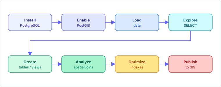From install to published map — every step in this post is a link in one repeatable chain.

From here, worthwhile directions include importing and exporting between more formats, triggers and functions for automated quality control, and the differences between PostGIS and ArcGIS Enterprise geodatabases.

The PostGIS and PostgreSQL communities are active — gis.stackexchange.com is a good place to work through real problems.

Full workshop materials, data, and setup instructions: learnspatialsql.com. Workshop by John Reiser.