SQL Data Cleaning for GIS

In GIS work, most of the effort goes into ETL — Extract, Transform, Load — before any mapping or analysis happens. Raw data almost always arrives dirty: mixed capitalization, blank cells, placeholder text like N/A, numbers stored as text, and inconsistent categories.

This guide is written for one specific stack, and each tool has a fixed job in it:

• GDAL (ogrinfo, ogr2ogr) — inspect files, load them into the database, reproject, and build geometry. It is the import/export layer.
• PostgreSQL / PostGIS — the cleaning and analysis layer. All real cleaning, type conversion, recoding, and spatial work happens here, using SQL.
• QGIS — the visualization layer. Connect it to PostGIS to view, style, and inspect the cleaned result.

The pattern throughout is the same: load raw data into PostGIS untouched, clean it with SQL, then view it in QGIS. Every example below is complete and runnable.

The workflow at a glance

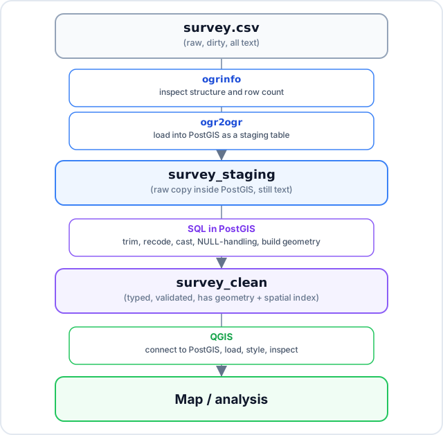The ETL pipeline: GDAL loads the raw file, PostGIS does the cleaning, QGIS displays the result.

The division of labor:

Tool	Job in this stack
GDAL (ogr2ogr)	Read the file, load it into PostGIS, reproject, build geometry from coordinates, export results.
PostgreSQL / PostGIS	All cleaning: whitespace, case, NULLs, type conversion, recoding, regex, joins, deduplication, spatial operations, constraints, indexes.
QGIS	Connect to the cleaned PostGIS table; view, style, inspect, and produce maps.

ogr2ogr can run limited SQL during import, but its native SQL dialect is small. In this stack there is no reason to fight it: load the raw file, then do every real transformation in PostGIS, where the full SQL toolkit lives.

The messy file we will clean

Assume the source is survey.csv:

id	name	depth	result	x	y
1	john smith	10	act nest	82311	451122
2	Mary Jones		INC NEST	82450	451090
3	PETER BROWN	15.5	suc nest	82502	451210
4	Anna White	N/A	ACT Nest	82333	451155
5	Bob Green	12		82388	451044

The result column holds survey status codes. For this guide, assume they mean: act = active, inc = inactive, suc = successful (these are domain-specific; substitute your own). The x / y columns are projected coordinates in meters.

The problems in this file:

• Mixed case in name and result.
• A blank cell in depth (row 2) and in result (row 5).
• N/A used as a placeholder in depth (row 4) instead of a true empty value.
• Inconsistent spelling/case in the categories (act nest, ACT Nest, INC NEST…).
• Coordinates are stored as plain columns, not yet a spatial geometry.

The single most important concept: a CSV has no data types

In a CSV, every value is text. There are no numbers, no dates, and no NULLs — only strings. This one fact explains most of the cleaning operations that follow.

Concretely, when ogr2ogr reads survey.csv into PostGIS, unless told otherwise every column arrives as text:

• The depth value 10 is the text "10", not the number 10.
• The blank cell in row 2 is an empty string "" — a string of length zero. It is not NULL.
• The value N/A in row 4 is the literal three-character string "N/A". The database has no idea it is meant to signal “missing”.
• The coordinates 82311 and 451122 are text, so they must be converted to numbers before building a point.

Consequences you will see repeatedly:

1. To do math on a column, you must first convert the text to a number (CAST).
2. To signal “missing”, you must replace empty strings and placeholders with real NULLs (NULLIF).
3. Comparing a column to '' or 'N/A' is comparing text to text — which is exactly why it works.

Keeping the data as text in the staging table is deliberate: it lets you clean each value explicitly instead of letting the importer guess types and fail on the dirty rows.

Step 1 — Inspect before you touch anything (ogrinfo)

Never load data you have not looked at. ogrinfo reports the structure and contents of a file.

# Summary only: layer name, field names + types, and feature (row) count
ogrinfo -so -al survey.csv

# Full dump: every field of every record
ogrinfo -al survey.csv

What to look for in the summary output:

• Field types are all String. This confirms the “everything is text” rule for CSV.
• Feature Count tells you how many rows you have, so you can verify nothing is lost after cleaning.
• The exact field names (they may be poorly named, like usr, dep, res), so you know what to rename.

Step 2 — Load the raw CSV into PostGIS

First, create the database and enable the PostGIS extension (once per database):

createdb gis
psql -d gis -c "CREATE EXTENSION IF NOT EXISTS postgis;"

Then load the raw file into a staging table with ogr2ogr. Keep the values as text; do not build geometry yet — that happens during cleaning.

ogr2ogr -f "PostgreSQL" \
    PG:"host=localhost port=5432 dbname=gis user=postgres password=secret" \
    survey.csv \
    -nln survey_staging \
    -oo EMPTY_STRING_AS_NULL=YES \
    -overwrite

Reading the flags:

• -f "PostgreSQL" — the output format (driver) is a PostgreSQL/PostGIS database.
• PG:"…" — the connection string: host, port, database, user, password.
• survey.csv — the input file.
• -nln survey_staging — new layer name: the destination table is survey_staging.
• -oo EMPTY_STRING_AS_NULL=YES — an open option for the CSV reader: turn blank cells into NULL on read. This does the work of Case 7 automatically for empty cells.
• -overwrite — replace the table if it already exists, so re-runs are safe.

After this, survey_staging holds an exact, still-messy copy of the CSV inside PostGIS. All cleaning now happens in SQL.

The cleaning operations

Every operation below runs in PostgreSQL/PostGIS against the staging table (named survey in the short examples for readability; it is survey_staging in the full pipeline).

Group A — Selecting and renaming columns

Case 1 — Rename fields with AS

Source columns are often cryptic. Suppose the file’s real column names are usr, dep, res. AS gives each output column a clear name. It renames the output; it does not change the source.

SELECT
    usr AS surveyor,
    dep AS depth,
    res AS result
FROM survey;

usr → surveyor	dep → depth	res → result
john smith	10	act nest

Selecting only the columns you want (instead of SELECT *) is also how you drop columns you do not need.

Group B — Normalizing text case

Case 2 — Uppercase with UPPER()

UPPER(text) converts every letter to uppercase. Useful for standardizing codes and categories.

SELECT UPPER(name) AS name
FROM survey;

Input	Output
john smith	JOHN SMITH
PETER BROWN	PETER BROWN

Case 3 — Lowercase with LOWER()

LOWER(text) does the reverse.

SELECT LOWER(result) AS result
FROM survey;

Input	Output
ACT NEST	act nest
SUC NEST	suc nest

Case 4 — Title Case with INITCAP()

INITCAP(text) capitalizes the first letter of each word and lowercases the rest.

SELECT INITCAP(name) AS name
FROM survey;

Input	Output
john smith	John Smith
PETER BROWN	Peter Brown

Caveat: INITCAP treats any non-letter as a word boundary, so mcdonald becomes Mcdonald (not McDonald) and o'brien becomes O'Brien. For personal names this is usually acceptable; for values where it is not, recode them explicitly with CASE (see Case 19).

Group C — Cleaning whitespace

Case 5 — Remove leading/trailing spaces with TRIM()

TRIM(text) removes spaces from the start and end of a value (not the middle).

SELECT TRIM(name) AS name
FROM survey;

Input	Output
" John Smith "	"John Smith"

Related: LTRIM() and RTRIM() trim only the left or right side. You can also trim specific characters, e.g. TRIM(BOTH '.' FROM code) removes leading/trailing dots.

Case 6 — Collapse internal multiple spaces with REGEXP_REPLACE()

TRIM cannot fix spaces inside a value. A regular expression can.

SELECT REGEXP_REPLACE(name, '\s+', ' ', 'g') AS name
FROM survey;

Reading the arguments: search each name for \s+ (one or more whitespace characters), replace each match with a single space, and the 'g' flag means global — replace every match, not just the first.

Input	Output
John Smith	John Smith

A robust pattern combines both whitespace fixes: TRIM(REGEXP_REPLACE(name, '\s+', ' ', 'g')).

Group D — Handling missing values (empty string vs N/A vs NULL)

Recall from the “everything is text” section: a blank cell is an empty string "", and N/A is a literal string. Neither is a true NULL. (If you used -oo EMPTY_STRING_AS_NULL=YES at import, empty cells are already NULL; the NULLIF for '' below is then a harmless safety net.)

Case 7 — Turn empty strings into NULL with NULLIF()

NULLIF(a, b) returns NULL if a equals b, otherwise returns a. Compare the column to the empty string:

SELECT NULLIF(depth, '') AS depth
FROM survey;

Input	Output
10	10
(blank)	NULL

Case 8 — Turn N/A into NULL

Same function, different comparison value:

SELECT NULLIF(depth, 'N/A') AS depth
FROM survey;

Input	Output
N/A	NULL

Handling several placeholders at once: nest the calls so both empty strings and N/A become NULL.

SELECT NULLIF(NULLIF(depth, ''), 'N/A') AS depth
FROM survey;

The inner NULLIF runs first (turning '' into NULL), and the outer one turns 'N/A' into NULL. Anything else passes through unchanged.

Case 9 — Replace NULL with a default using COALESCE()

COALESCE(a, b, …) returns the first argument that is not NULL. Use it to show a value instead of a blank.

SELECT COALESCE(result, 'Unknown') AS result
FROM survey;

Input	Output
ACT NEST	ACT NEST
NULL	Unknown

Order matters: NULLIF creates NULLs from placeholders; COALESCE replaces NULLs with a value. You often use NULLIF first, then COALESCE.

Group E — Working with numbers

Case 11 — Convert text to a number with CAST()

Because staged values are text, you must convert before doing math or numeric comparisons.

SELECT CAST(depth AS REAL) AS depth
FROM survey;

Input	Output
"15"	15.0

PostgreSQL also offers a shorthand: depth::REAL.

Critical ordering: CAST('N/A' AS REAL) throws an error, because N/A is not a number. Always clean placeholders to NULL first, then cast:

SELECT NULLIF(NULLIF(depth, ''), 'N/A')::REAL AS depth
FROM survey;

NULL casts to a numeric NULL without error, so this succeeds on every row.

Case 10 — Round with ROUND()

ROUND(number, decimals) rounds to the given number of decimal places. (NUMERIC supports the two-argument form; cast text to NUMERIC first.)

SELECT ROUND(NULLIF(NULLIF(depth, ''), 'N/A')::NUMERIC, 1) AS depth
FROM survey;

Input	Output
10.347	10.3

Case 12 — Create a new (derived) column

Compute new columns from existing ones. Here, convert meters to feet (1 m = 3.28084 ft):

SELECT
    NULLIF(NULLIF(depth, ''), 'N/A')::REAL              AS depth_m,
    NULLIF(NULLIF(depth, ''), 'N/A')::REAL * 3.28084    AS depth_ft
FROM survey;

depth_m	depth_ft
10.0	32.8084
15.5	50.85302

Group F — Filtering rows

Case 13 — Keep only valid rows with WHERE

WHERE decides which rows are returned. Keep only positive depths:

SELECT *
FROM survey
WHERE NULLIF(NULLIF(depth, ''), 'N/A')::REAL > 0;

Two beginner traps here:

1. depth is text, so it is cleaned and cast before the > comparison.
2. Comparisons with NULL are never true. After cleaning, the blank and N/A rows are NULL, and NULL > 0 is “unknown”, so those rows are excluded. If you want to keep them, add OR depth IS NULL.

Group G — Recoding and standardizing categories

Case 14 — Translate codes with CASE

CASE is SQL’s if/else. It checks conditions in order and returns the matching value.

SELECT
    CASE
        WHEN result = 'A' THEN 'Active'
        WHEN result = 'I' THEN 'Inactive'
        WHEN result = 'S' THEN 'Successful'
        ELSE 'Unknown'
    END AS result
FROM survey;

Input	Output
A	Active
I	Inactive
S	Successful
(anything else)	Unknown

Always include ELSE. Without it, any value that matches no WHEN returns NULL — a common source of surprise blanks.

Case 19 — Standardize messy category variants

Real category columns contain the same meaning written many ways: Act Nest, ACT NEST, act nest, Active Nest. Collapse them to one canonical value. Normalize case and whitespace first, then map:

SELECT
    CASE
        WHEN UPPER(TRIM(result)) IN ('ACT NEST', 'ACTIVE NEST')      THEN 'ACT NEST'
        WHEN UPPER(TRIM(result)) IN ('INC NEST', 'INACTIVE NEST')    THEN 'INC NEST'
        WHEN UPPER(TRIM(result)) IN ('SUC NEST', 'SUCCESSFUL NEST')  THEN 'SUC NEST'
        ELSE NULL
    END AS result
FROM survey;

Applying UPPER(TRIM(...)) before comparing means you write each condition once instead of listing every capitalization.

Group H — Combining and splitting text

Case 15 — Join fields with ||

|| is the string concatenation operator. Build a full name from two columns:

SELECT first_name || ' ' || last_name AS full_name
FROM survey;

first_name	last_name	full_name
John	Smith	John Smith

NULL trap: 'John' || NULL is NULL — one NULL poisons the whole result. Use concat_ws instead, which skips NULLs and inserts the separator only between present values:

-- concat_ws = "concatenate with separator"
SELECT concat_ws(' ', first_name, last_name) AS full_name
FROM survey;

Case 16 — Split a field with SPLIT_PART()

SPLIT_PART(text, delimiter, n) returns the n-th piece after splitting on the delimiter.

SELECT
    SPLIT_PART(name, ' ', 1) AS first_name,
    SPLIT_PART(name, ' ', 2) AS last_name
FROM survey;

Input	first_name	last_name
John Smith	John	Smith

Caveat: position-based splitting is fragile for names with middle names or more than two words. Handle those cases explicitly if your data contains them.

Group I — Dates

Case 17 — Parse a text date with TO_DATE()

CSV dates are text in whatever format the source used. TO_DATE(text, format) converts them to a real DATE. You must describe the input format.

-- Interprets the text as day/month/2-digit-year
SELECT TO_DATE('01/07/26', 'DD/MM/YY') AS survey_date;

Input	Output (ISO DATE)
01/07/26	2026-07-01

Two real-world traps:

1. Ambiguity. 01/07/26 is July 1st under DD/MM/YY but January 7th under MM/DD/YY. The format string decides — you must know which convention the source used.
2. Two-digit years. 26 could be 1926 or 2026. Prefer sources with 4-digit years (YYYY) whenever possible.

Group J — Removing duplicates

Case 18 — Drop identical rows with DISTINCT

SELECT DISTINCT removes rows that are duplicates across all selected columns.

SELECT DISTINCT *
FROM survey;

When this is not enough: if two rows share the same id but differ elsewhere, DISTINCT * keeps both because the rows are not identical. To keep one row per key, use a window function:

-- Keep the first row per id, ordered by depth
SELECT id, name, depth, result
FROM (
    SELECT *,
           ROW_NUMBER() OVER (PARTITION BY id ORDER BY depth) AS rn
    FROM survey
) AS numbered
WHERE rn = 1;

ROW_NUMBER() OVER (PARTITION BY id …) numbers the rows within each id group; keeping rn = 1 returns one row per id.

Group K — Building geometry and handling CRS in PostGIS

Case 20 — Turn X/Y columns into a point geometry

A point geometry is written internally from its X and Y coordinates. Because the staged x/y are text, cast them to numbers, build the point, and stamp it with a coordinate reference system (CRS).

Two functions do the work:

• ST_MakePoint(x, y) — builds the point from numeric coordinates. At this stage the point has no CRS.
• ST_SetSRID(geometry, srid) — records which CRS the coordinates are in, using an SRID (the numeric part of an EPSG code).

The large coordinate values here (tens of thousands) indicate a projected CRS in meters, not longitude/latitude. Use the correct EPSG code for your data — the example uses 32631 (UTM zone 31N).

SELECT
    id,
    ST_SetSRID(ST_MakePoint(x::REAL, y::REAL), 32631) AS geom
FROM survey;

Assign vs. transform — a key distinction:

• ST_SetSRID(geom, 32631) declares the CRS. It only records what the coordinates already are; it does not move any point.
• ST_Transform(geom, 4326) reprojects — it recalculates the coordinates into a different CRS. It requires the geometry to already have a correct SRID set.

Example: build the point in UTM, then reproject to WGS84 longitude/latitude (EPSG:4326):

SELECT
    id,
    ST_Transform(ST_SetSRID(ST_MakePoint(x::REAL, y::REAL), 32631), 4326) AS geom_wgs84
FROM survey;

The same distinction exists on the GDAL side: ogr2ogr -a_srs assigns a CRS without moving points, while ogr2ogr -t_srs transforms coordinates into a target CRS. Mixing them up (declaring the wrong CRS, or transforming from a wrong source) puts data in the wrong place on the map.

Complete end-to-end pipeline

This is the full sequence from an empty database to a styled QGIS layer, using the sample survey.csv (columns id, name, depth, result, x, y). Every command is shown in full.

1. Create the database and enable PostGIS (once per database):

createdb gis
psql -d gis -c "CREATE EXTENSION IF NOT EXISTS postgis;"

2. Inspect the raw file:

ogrinfo -so -al survey.csv

3. Load the raw CSV into a staging table (values kept as text, blanks → NULL):

ogr2ogr -f "PostgreSQL" \
    PG:"host=localhost port=5432 dbname=gis user=postgres password=secret" \
    survey.csv \
    -nln survey_staging \
    -oo EMPTY_STRING_AS_NULL=YES \
    -overwrite

4. Clean and build geometry in one query, storing the result as a new table. Run this in psql -d gis or QGIS DB Manager:

DROP TABLE IF EXISTS survey_clean;

CREATE TABLE survey_clean AS
SELECT
    CAST(id AS INTEGER)                                          AS id,        -- text → integer key
    INITCAP(TRIM(name))                                         AS surveyor,  -- trim, then Title Case
    NULLIF(NULLIF(depth, ''), 'N/A')::REAL                      AS depth,     -- placeholders → NULL, then → number
    UPPER(TRIM(result))                                        AS result,    -- trim, then a consistent uppercase code
    ST_SetSRID(ST_MakePoint(x::REAL, y::REAL), 32631)          AS geom       -- build point in EPSG:32631
FROM survey_staging;

5. Add a primary key and a spatial index. Both matter for the next step: QGIS loads PostGIS tables best when there is an integer primary key, and the GIST index speeds up rendering and spatial queries.

ALTER TABLE survey_clean ADD PRIMARY KEY (id);
CREATE INDEX survey_clean_geom_idx ON survey_clean USING GIST (geom);

6. (Optional) Export the cleaned table to a GeoPackage for sharing outside the database:

ogr2ogr -f "GPKG" survey_clean.gpkg \
    PG:"host=localhost port=5432 dbname=gis user=postgres password=secret" \
    survey_clean

The cleaned result:

id	surveyor	depth	result	geom
1	John Smith	10.0	ACT NEST	POINT(82311 451122)
2	Mary Jones	NULL	INC NEST	POINT(82450 451090)
3	Peter Brown	15.5	SUC NEST	POINT(82502 451210)
4	Anna White	NULL	ACT NEST	POINT(82333 451155)
5	Bob Green	12.0	(empty)	POINT(82388 451044)

Reading the cleaning query against the output: id becomes a real integer; TRIM + INITCAP fixes the names; the nested NULLIF turns '' and N/A into NULL and ::REAL converts the survivors to numbers; TRIM + UPPER normalizes the status codes; and ST_MakePoint + ST_SetSRID builds a proper point geometry in EPSG:32631.

Load the result in QGIS

With survey_clean cleaned, indexed, and keyed, connect QGIS to the database:

1. Open Layer → Data Source Manager → PostgreSQL (or the Add PostGIS Layers button).
2. Create a new connection with the same host, port, database, and user used in the ogr2ogr command.
3. Expand the connection, select survey_clean, and add it to the map.

Two practical notes for this stack:

• QGIS needs a unique integer column to load a PostGIS table reliably. The PRIMARY KEY (id) added in step 5 provides it; without a key, QGIS may refuse the layer or behave unpredictably during editing.
• The GIST spatial index added in step 5 keeps rendering and identify/select operations fast as the table grows.

QGIS can also run SQL directly against PostGIS through Database → DB Manager → SQL Window, which is convenient for testing cleaning queries before saving them as a table.

Recommended order of operations

The order of cleaning steps matters, because later steps assume earlier ones have run. A reliable sequence inside PostGIS:

1. Trim whitespace (TRIM, REGEXP_REPLACE) — so later comparisons and case conversions see clean text.
2. Normalize case (UPPER / LOWER / INITCAP) — so category matching is consistent.
3. Convert placeholders to NULL (NULLIF) — turn '' and N/A into real missing values.
4. Cast types (CAST) — only after placeholders are NULL, or the cast will error.
5. Round and derive (ROUND, arithmetic) — now that values are numeric.
6. Recode categories (CASE) — map cleaned text to canonical values.
7. Filter rows (WHERE) — remembering that NULLs drop out of numeric comparisons.
8. Build geometry (ST_MakePoint + ST_SetSRID, then ST_Transform if reprojecting).
9. Add constraints and indexes (PRIMARY KEY, GIST) — for validation and QGIS performance.

The two orderings that break most often for beginners: casting before nullifying placeholders (errors on N/A), and comparing/recoding before trimming and normalizing case (misses variants).

Summary of the stack pattern

• GDAL loads and moves data. Use ogrinfo to inspect and ogr2ogr to load the raw file into a PostGIS staging table untouched. Use -a_srs to declare a CRS and -t_srs to reproject.
• PostGIS does the cleaning. Every real transformation — whitespace, case, NULL handling, type conversion, recoding, geometry construction, deduplication — is SQL run against the staging table, producing a clean table with constraints and a spatial index.
• QGIS visualizes the result. Connect to PostGIS and load the cleaned, keyed, indexed table for styling, inspection, and map production; use DB Manager to prototype SQL.

For one-off datasets this whole sequence is a handful of commands. For recurring workflows, save the cleaning SQL as a script (or a view) so re-running it on new data is a single step.